- Wachter Space Blog about Security and Automated Methods/
- Posts/
- Machine Learning for Computer Security at KIT/
Machine Learning for Computer Security at KIT
Table of Contents
Overview #
The mind map below summarizes topics from the lecture. I use mind maps like this at the start of exam preparation to see what I remember from the semester. While studying, I expand on the topics. Later, I color-code the nodes to show which topics I know well and which ones I still need to practice.
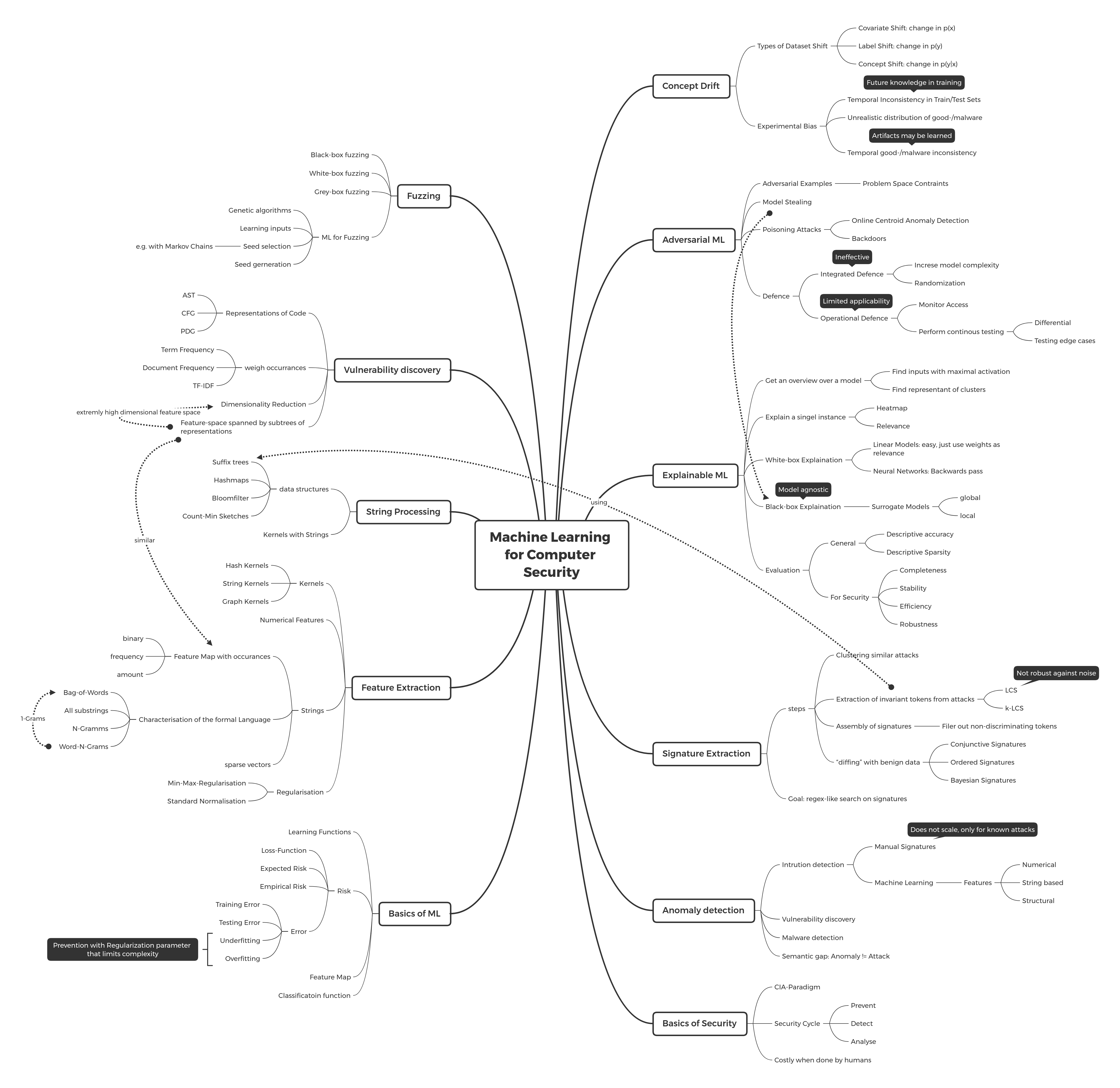
I also made an Anki deck, but unfortunately it contains screenshots of lecture slides that are not released under a free license.
Exam practice questions #
Introduction #
What are the three main security goals?
Click to view answer
Confidentiality, integrity, and availability: the CIA triad. These are general goals that need concrete definitions for a particular system. Other goals, such as authenticity and accountability, may also be relevant.
Describe the inverse feature-mapping problem.
Click to view answer
A feature map takes a sample from problem space into feature space. This direction is usually straightforward, but reversing it can be difficult or impossible. The map may discard information or map several samples to the same vector, so the original sample cannot always be recovered uniquely. Even finding any valid sample with a specified feature vector can be difficult because of constraints in problem space. This complicates the study of adversarial examples.
Which stages make up the security cycle described in the lecture? Why is there an imbalance? Name an automation technique from the lecture and explain where it helps.
Click to view answer
The cycle discussed in the lecture consists of prevention, detection, and analysis. The volume and diversity of new malware and attacks exceed the capacity of human analysts, creating a need for automation.
Fuzzing automates parts of vulnerability discovery, although setting up a useful fuzzing campaign can still require human effort. Finding and fixing vulnerabilities before attackers exploit them contributes to prevention.
What challenges arise when applying machine learning to computer security?
Click to view answer
- Effectiveness: A high detection rate with few false positives.
- Efficiency: The ability to process large amounts of data with reasonable computational cost.
- Robustness: Resistance to evasion, unusual inputs, and changes in the data distribution.
Machine Learning 101 #
What are training, validation, and test sets? What requirements should they satisfy?
Click to view answer
A model’s parameters are fitted using the training set. The test set is held out for evaluating the model’s performance on unseen data. Hyperparameters should be selected using separate validation data or cross-validation, rather than the test set.
The sets must be disjoint, and information must not leak between them through duplicate samples, preprocessing, or related observations. For an evaluation intended to reflect future deployment, training data should precede test data in time. Otherwise, we risk “learning the future and predicting the past”. The concept-drift section discusses further requirements for security datasets.
What is a loss function? Give three examples. For which task is binary hinge loss suitable, and which labels does it require?
Click to view answer
A loss function measures the error of a prediction relative to the true target. Three examples are:
-
Hinge loss, for a binary classification score :
-
0–1 loss, for a predicted class label :
-
Squared loss, commonly used for regression:
The binary hinge-loss formula assumes labels . Its first argument is a real-valued score, rather than just the predicted class label.
What is underfitting? What is overfitting? Give an example of how to constrain the complexity of a model.
Click to view answer
Underfitting occurs when a model is too restrictive to capture relevant patterns, resulting in poor performance even on the training data. Overfitting occurs when a model fits noise or sample-specific details and performs substantially worse on unseen data.
Empirical risk minimization alone seeks:
This can lead to overfitting, particularly with a flexible model and limited data. One way to constrain complexity is to add a regularization term:
Here, penalizes complexity, for example through a squared weight norm. The parameter controls the trade-off between fitting the training data and limiting complexity. It can be selected using validation data.
What is expected risk, and how can it be estimated?
Click to view answer
Expected risk is the expected loss under the joint distribution of inputs and targets:
Since this distribution is usually unknown, we estimate the risk using the average loss on a sample:
This is the empirical risk. Its usefulness as an estimate depends on how the samples and model were selected.
Does low empirical risk imply low expected risk? What issue can arise? How can this issue be mitigated?
Click to view answer
No. A model can have low training loss while overfitting the training set and generalizing poorly. Expected risk averages over the underlying distribution; training empirical risk uses only the observed training samples.
Representative data, suitable complexity control, and independent validation help reduce this problem. An untouched test set estimates generalization performance after model selection. Regularization reduces overfitting risk but does not guarantee low expected risk.
Given a labeled dataset , explain -fold cross-validation. Draw a sketch for .
Click to view answer
Split the training dataset into roughly equal folds. For each candidate hyperparameter setting, train a fresh model on folds and validate it on the remaining fold. Rotate the held-out fold so that every fold is used for validation once. Select the setting with the best average validation score, then refit on the full training dataset.
For :
| Run | Fold 1 | Fold 2 | Fold 3 | Fold 4 |
|---|---|---|---|---|
| 1 | Validate | Train | Train | Train |
| 2 | Train | Validate | Train | Train |
| 3 | Train | Train | Validate | Train |
| 4 | Train | Train | Train | Validate |
The final test set remains separate throughout model selection. Preprocessing must also be fitted within each training fold. Temporal or grouped data require splits that respect those dependencies, rather than ordinary random folds. See the cross-validation documentation.
Are XOR, AND, and OR linearly separable? Why or why not?
Click to view answer
For binary inputs , XOR is not linearly separable: its positive and negative examples occupy opposite corners of the square, so no single straight line separates them.
AND and OR are linearly separable. For example, classify an input as positive when for AND, or when for OR. Linear independence of the three points in one class is not required.
How do discriminative and generative models differ? How does this relate to supervised and unsupervised learning? Give security-related examples.
Click to view answer
Discriminative models learn a decision function or model directly. Generative classifiers model the joint distribution , often through and , and use it to infer a label. Generative models can also model unlabeled observations through .
This distinction is separate from supervised versus unsupervised learning, which concerns the availability of labels. Both generative and discriminative classifiers can be trained on labeled data; naive Bayes is a generative classifier, while logistic regression is discriminative. See Ng and Jordan’s comparison.
In security, supervised models can classify benign and malicious programs. When representative attack labels are unavailable, unsupervised or one-class methods can model normal activity for anomaly detection. An anomaly is not automatically an attack.
From Data to Features #
How are strings mapped into feature space? Define an occurrence-based feature map and explain how its vocabulary can be constructed.
Click to view answer
Choose a vocabulary , such as words obtained by tokenization, character -grams, or selected substrings. Define an occurrence function that records whether token occurs in sample , how often it occurs, or its relative frequency. With token weights , the feature map is:
The vocabulary and weights must be chosen consistently across samples.
What are the advantages and disadvantages of feature hashing?
Click to view answer
Feature hashing maps tokens to a fixed number of feature indices without storing an explicit vocabulary. This makes the representation compact and suitable for large or changing vocabularies.
Collisions merge information from different tokens, and individual dimensions are harder to interpret. For example, buckets give a fixed feature-space dimension of ; a larger space, such as , trades memory for fewer collisions. An appropriate size depends on the dataset.
Hashing does not preserve numerical proximity: small changes to a token can send it to a completely different bucket. Continuous values therefore need an appropriate representation rather than simply being hashed as strings.
How does feature scaling help? Give formulas for two approaches.
Click to view answer
Feature scales and offsets can differ substantially. Scaling prevents a few large-valued features from dominating distance calculations or optimization merely because of their units.
Standardization subtracts the mean and divides by the standard deviation:
Min–max scaling maps the training range to :
Fit the scaling parameters on training data and reuse them for validation and test data. Constant features require special handling because their denominators are zero. Values outside the training range can fall outside after min–max scaling.
Describe methods of extracting features from strings. Give examples that require word tokenization and examples that do not.
Click to view answer
With a tokenizer or known delimiter:
- Bag of words (word unigrams): Split the input into words and record their occurrences. This loses word order.
- Word -grams: Extract sequences of consecutive words, retaining some local context.
Without word delimiters:
- All substrings: Consider every contiguous substring. This retains context but creates a large, redundant vocabulary.
- Character or byte -grams: Extract contiguous substrings of a fixed length .
What properties must a function have to be a valid real-valued kernel?
Click to view answer
A real-valued kernel has the form . It must be symmetric, and every finite Gram matrix must be positive semidefinite. Equivalently, for every finite collection and real coefficients :
Such a kernel can be represented as an inner product in a feature space, which may be infinite-dimensional.
Show that:
Click to view answer
Using , expand the squared norm:
Taking the nonnegative square root proves the identity. This inner-product argument also works in an infinite-dimensional feature space.
What makes a kernel function so useful?
Click to view answer
The kernel trick evaluates inner products in a feature space without explicitly computing the feature vectors:
Algorithms expressed through inner products can therefore learn nonlinear decision boundaries in the original input space. Some kernels correspond to infinite-dimensional feature spaces. Choosing a kernel does not, by itself, guarantee that a particular dataset becomes separable.
Compute the similarity between “implementation” and “installation” using character bigrams, binary occurrence features, unit weights, and the dot product.
Click to view answer
For a="implementation", the distinct character bigrams are:
A={im,mp,pl,le,em,me,en,nt,ta,at,ti,io,on}.
For b="installation", they are:
B={in,ns,st,ta,al,ll,la,at,ti,io,on}.
The intersection is A∩B={ta,at,ti,io,on}. With binary occurrence features and all weights equal to 1:
Why can simple numerical summaries be insufficient for security data?
Click to view answer
Simple numerical summaries, such as length or entropy, can miss the ordering and relationships that distinguish security-relevant structures. Richer representations can encode strings, syntax, control flow, or data dependencies. These representations may still be mapped to numerical feature vectors; the limitation is in the information captured, rather than in numbers themselves.
String Processing #
Explain a Count-Min Sketch. How are counts updated and estimated? What guarantee holds for nonnegative updates?
Click to view answer
A Count-Min Sketch estimates item frequencies using several arrays of counters and independent hash functions. For unit insertions, update one counter in each array:
Estimate the frequency using the smallest of those counters:
With nonnegative updates and no counter overflow, collisions can increase counts but cannot decrease them. The estimate therefore never underestimates the true count, although it may overestimate it.
What is the difference between a Bloom filter and a Count-Min Sketch?
Click to view answer
A Bloom filter approximates set membership: “Has this item been inserted?” A standard Bloom filter uses a bit array and several hash functions. It can produce false positives but, without deletions, does not produce false negatives.
A Count-Min Sketch estimates frequencies: “How many times has this item been inserted?” It typically uses one counter array per hash function. Under nonnegative updates, its estimates can be too high but not too low.
What makes suffix trees the Swiss Army knife of string analysis?
Click to view answer
Suffix trees support many string-processing operations within one data structure, including substring searches, longest common substrings (LCS), -common substrings (KCS), and some string-kernel computations. They can be constructed in linear time under the usual fixed-alphabet assumptions.
Why can the longest common substring (LCS) be sensitive to noisy datasets? Give an example and explain an alternative.
Click to view answer
A longest common substring shared by all samples is sensitive to noise. A single unrelated or incomplete sample can shorten the result substantially, even if the other samples share a long substring. For example:
A common sequencenoiseA common sequenceA common sequence
The longest substring shared by all four is se. A -common substring approach instead considers substrings shared by at least distinct samples. Choosing allows the longer common text to be recovered despite the noisy sample. Here, is a minimum number of samples, not a number of tokens to extract. See Gusfield’s treatment of common substrings.
Name three different kinds of signatures.
Click to view answer
- Conjunctive signatures: Require several tokens to be present.
- Bayesian signatures: Combine token evidence using probabilistic scores.
- Ordered signatures: Require tokens to occur in a specified order.
Name at least one way in which an attacker can make the signature generation algorithm less effective.
Click to view answer
If the training data can be influenced, poisoning can introduce misleading associations between features and labels. Signature generation can also overfit incidental tokens that are shared by the observed samples but are not essential to their malicious behavior. Such tokens may disappear in later variants.
What are common steps in signature generation?
Click to view answer
- Cluster related attack samples.
- Extract shared or invariant tokens.
- Select tokens that discriminate between malicious and benign samples.
- Assemble signatures that can be matched against new data.
Are signatures robust?
Click to view answer
Their robustness depends on what they capture. A signature based on incidental byte sequences can fail when those sequences change. A signature based on more stable properties may cover multiple variants, but it can still suffer from poisoning, incomplete training data, or changes in malicious behavior. Robustness must be evaluated rather than assumed.
Anomaly Detection #
Which types of features were discussed in the lecture? Give examples.
Click to view answer
- Numerical features: For example, length and entropy.
- String features: For example, tokens or byte sequences from a protocol message.
- Structured features: For example, patterns in abstract syntax trees (ASTs) or code property graphs (CPGs).
Given benign training data , state the minimum-hypersphere (SVDD) optimization problem. How can slack variables reduce sensitivity to outliers?
Click to view answer
The hypersphere formulation is support vector data description (SVDD), a method for one-class classification. For training samples , the hard formulation minimizes the squared radius:
Outliers can force the sphere to become very large. Introduce nonnegative slack variables to allow some training samples outside the sphere while penalizing those violations:
Here, controls the penalty for violations. Slack variables reduce the influence of outliers but do not guarantee robustness to arbitrary contamination.
How does the SVM penalty parameter affect the solution? How does its role differ from a regularization weight ?
Click to view answer
Specify which parameter is meant. In the usual soft-margin objective,
a larger penalizes margin violations more strongly, while a smaller permits more violations in exchange for a smaller weight norm. Describing this merely as a “sharp” or “soft” decision boundary is imprecise.
In an objective written as empirical loss plus , increasing instead strengthens regularization. See the SVM formulation.
Describe three different approaches for learning-based attack detection.
Click to view answer
- Model benign behavior and flag deviations.
- Model known malicious behavior and recognize similar activity.
- Learn a boundary between labeled benign and malicious samples.
What assumptions are made for anomaly detection?
Click to view answer
Anomaly detection assumes that a model of normal behavior can identify meaningful deviations. Training data should represent normal activity and, depending on the method, be benign or predominantly benign.
There is a semantic gap: unusual behavior is not necessarily malicious, and malicious behavior is not necessarily unusual. When reliable attack labels are unavailable, unsupervised or one-class methods can be useful, but their alerts still require interpretation.
Which geometric approaches can be used to model normality?
Click to view answer
Global centroid models, hypersphere-based one-class models such as SVDD, and local neighborhood-based models. The first uses a single global center; local models compare a sample with nearby observations.
Give the centroid formula for a global model of normality and explain its meaning.
Click to view answer
The global center is the mean of the training feature vectors:
A simple model chooses a radius around this point that encloses the training samples. Samples outside the radius are flagged as anomalous. Both the mean and a radius chosen to cover every sample can be sensitive to outliers.
Give a distance-based anomaly score for a centroid model.
Click to view answer
The squared distance from the center is:
Larger values indicate greater deviation from the modeled center. A threshold is needed to turn the score into a decision.
What are the drawbacks of signatures?
Click to view answer
Signatures can miss new attacks or variants that no longer contain the properties they match. Creating and distributing updated signatures also introduces delay and maintenance costs.
This does not mean that every signature fails on every variation: signatures based on stable properties can recognize families of related attacks. Their coverage depends on the signature and the changes in the samples.
Show that:
Click to view answer
Let and . Expanding the squared norm gives:
Malware Classification #
What assumptions underlie learning-based classification for attack detection?
Click to view answer
A two-class detector needs sufficiently large and representative samples of both benign and malicious activity. Generalization assumes that future observations share relevant patterns with the training data.
A model of benign behavior can identify deviations, but those deviations are not automatically malware. A model of known malware can recognize similarities to past attacks, but it may miss genuinely different behavior. These limitations are part of the semantic gap between statistical patterns and security judgments.
Which sources can provide samples for machine-learning-based malware classification? What limitations do these sources have?
Click to view answer
Possible sources include manual analysis, antivirus detections, and sample repositories such as VirusTotal. These sources can be biased, incomplete, or missing reliable labels. Samples collected for convenience should not automatically be treated as representative of deployment data.
Define the perceptron decision rule and its learning updates.
Click to view answer
For labels , the decision rule is:
with a fixed convention for a zero score. The perceptron repeatedly visits the training samples. If
it updates both the weights and the bias:
where is the learning rate. Equivalently, the bias can be included in an augmented weight vector with a constant input feature. For a finite, linearly separable training set, the standard perceptron converges to a separating classifier; nonseparable data do not have this guarantee.
Define the decision rule and optimization problems for hard-margin and soft-margin two-class SVMs.
Click to view answer
For a two-class SVM, the decision rule is:
For separable training data with labels , the hard-margin problem is:
For nonseparable data, the soft-margin problem allows margin violations through slack variables:
The label multiplies the entire decision score, including the bias. A kernel changes the feature space; it does not guarantee separability. See the standard mathematical formulation.
Give examples of attacks against classification methods.
Click to view answer
- Poisoning during learning: Contaminating training data or labels.
- Mimicry during detection: Making malicious activity resemble benign activity in the features used by the detector.
- Red herrings: Generating misleading alerts that consume analysis resources.
What are support vectors? How can outliers affect an SVM?
Click to view answer
Support vectors are training samples with nonzero coefficients in the SVM’s dual solution. They determine the decision boundary. In the hard-margin case, they lie on the margin boundaries. In the soft-margin case, they can also lie inside the margin or be misclassified.
Outliers can therefore influence the boundary, particularly when violations are penalized heavily. Soft margins help control this sensitivity, but support-vector methods are not automatically robust to arbitrary outliers.
How do one-class methods differ from two-class SVMs? Give typical applications.
Click to view answer
A two-class SVM uses labeled examples of two classes to learn a separating decision boundary with a large margin. A typical application is distinguishing known malware from benign programs.
A one-class method models one target class and identifies samples that do not fit it. A typical application is modeling benign behavior for anomaly detection. The standard one-class SVM uses a separating hyperplane in feature space; the lecture’s hypersphere picture corresponds to SVDD. A soft hypersphere formulation can leave some training samples outside the sphere.
Concept Drift #
What is concept drift, and how does it relate to dataset shift?
Click to view answer
Concept drift refers to changes in the data-generating process over time that can undermine a model’s predictions. The lecture uses the term broadly for changing data distributions.
Dataset shift is the more general mismatch between training and deployment distributions, whether or not it is caused by time. In the narrower terminology used below, concept shift changes . Terminology varies, so the changing distribution should always be stated explicitly.
What are the main types of dataset shift? Give one example for each. State the changing distribution.
Click to view answer
- Covariate shift: changes while stays fixed. For example, an API call becomes more common, while its relationship to maliciousness remains unchanged.
- Label shift: changes while stays fixed. For example, the proportion of malware increases while the within-class feature distributions remain unchanged.
- Concept shift: changes. For example, an SMS-related feature becomes less indicative of malware because benign applications increasingly use it.
The invariance assumptions distinguish these cases. See the original discussions of covariate shift and label shift.
How can dataset shift be addressed, particularly in a nonstationary domain?
Click to view answer
Active learning selects informative samples for labeling. Incremental learning or retraining updates a model as new data become available. These approaches need reliable labels or other safeguards against incorporating misleading data, and their effectiveness should be evaluated on appropriately time-ordered data.
What is the confusion matrix? Define precision and recall.
Click to view answer
A confusion matrix counts outcomes by their true and predicted classes:
| Actual class | Predicted positive | Predicted negative |
|---|---|---|
| Positive | True positive (TP) | False negative (FN) |
| Negative | False positive (FP) | True negative (TN) |
“Positive” and “negative” describe the prediction; “true” and “false” describe whether it is correct.
Precision measures how many positive predictions are correct. Recall measures how many actual positives are detected. If a denominator is zero, the corresponding ratio is undefined unless an evaluation convention specifies otherwise.
Is accuracy always a good metric?
Click to view answer
No. With imbalanced classes, a trivial classifier can achieve high accuracy while failing to detect the class of interest. For example, suppose of samples are benign. A classifier that always predicts “benign” achieves:
but its recall for malicious samples is zero. Evaluation should also consider class-specific metrics and the relative costs of errors.
What can cause concept drift or other forms of dataset shift?
Click to view answer
In the lecture’s broad use of the term, changing user behavior, software, or attack patterns can cause drift. Dataset shift can also arise from sampling or selection bias: the collected data may differ from the deployment population even without a temporal change.
Vulnerability Discovery #
Name graph-based representations of code.
Click to view answer
- Control-flow graph (CFG): Represents possible transfers of control.
- Program-dependence graph (PDG): Represents data and control dependencies.
- Abstract syntax tree (AST): Represents the syntactic structure of a program.
Rank the following terms by TF–IDF under an explicitly stated IDF definition. Explain the rationale behind TF–IDF.
- a word that is common in every document.
- a word that is not present in the current document, but in every other document.
- a word that only occurs in the current document.
Click to view answer
Specify the IDF convention first. With the unsmoothed definition
where is the number of documents:
- A term present in every document has IDF zero, so its TF–IDF is zero.
- A term absent from the current document has TF zero, so its TF–IDF is zero.
- A term present only in the current document has positive TF and maximal IDF, , so it receives a positive weight.
Under this convention, the first two cases tie at zero and the third ranks above them. Smoothed or offset IDF formulas can change these values and the ranking.
TF–IDF emphasizes terms that occur in a document but are uncommon across the collection, making them useful for distinguishing documents.
Briefly explain the Heartbleed vulnerability.
Click to view answer
I doubt that this will be an exam question, but briefly: Heartbleed was a missing bounds check in OpenSSL’s TLS heartbeat implementation. A supplied length could exceed the actual heartbeat payload, causing a buffer over-read that exposed process memory. Leaked data could include sensitive information such as private keys. See the OpenSSL security advisory.
Why do we apply dimensionality reduction?
Click to view answer
Dimensionality reduction can reduce storage and computational costs, remove redundancy, and sometimes suppress noise while retaining useful structure.
Principal component analysis (PCA) projects data onto directions of high variance. Low variance is not the same as irrelevance, so PCA can discard features that matter for a security task. The retained representation must be evaluated for the intended application.
What are the two approaches to vulnerability discovery mentioned in the lecture?
Click to view answer
- Find code patterns similar to those associated with known vulnerabilities.
- Identify abnormal code patterns that may indicate previously unknown vulnerabilities.
How can code be mapped to structural features? What is required for this mapping?
Click to view answer
Choose subtrees or subgraphs from a structural representation of code and map their occurrences to features:
This requires a code representation, such as an AST, CFG, PDG, or CPG; a consistent set of structural patterns ; an occurrence function; and weights. Occurrence values can encode term frequency (TF), while weights can encode inverse document frequency (IDF), giving TF–IDF features.
What is taint analysis? Can it be static or dynamic?
Click to view answer
Taint analysis tracks how data from specified sources, such as user input, can flow to security-critical sinks. It can help identify potentially unsafe uses of untrusted input, taking relevant checks or sanitization into account. Taint analysis can be performed statically, dynamically, or through a combination of both.
Fuzzing #
Classify fuzzers by how they generate inputs.
Click to view answer
- Generation-based: Construct inputs from a model or grammar.
- Mutation-based: Modify existing inputs.
- Evolutionary: Use feedback to select and evolve promising inputs, often through mutation.
These categories overlap: evolutionary fuzzers are often mutation-based.
How do black-box, grey-box, and white-box fuzzers differ? Compare their typical analysis overhead.
Click to view answer
- Black-box fuzzers use little or no information about the program’s internal structure.
- Grey-box fuzzers use lightweight feedback, such as coverage.
- White-box fuzzers, in the lecture’s terminology, use more detailed program reasoning, such as symbolic execution.
Detailed analysis generally costs more per generated test than lightweight feedback. The exact overhead depends on the implementation, so this is a tendency rather than an absolute ranking. AFL records approximate coverage in a bitmap; its parallel mode runs multiple fuzzer processes, rather than multiple threads within one instance. See the AFL documentation.
AFL can be viewed as an evolutionary algorithm. What feedback guides it?
Click to view answer
AFL rewards inputs that reveal new coverage information, including previously unseen edges or new hit-count categories. These inputs can be retained for further mutation.
“The number of newly covered edges” is a useful simplified description of the feedback, but AFL does not use that quantity alone as a single genetic-algorithm fitness score. Seed selection and mutation effort also consider other properties. See the technical documentation.
What is NEUZZ? What is the rough idea behind it?
Click to view answer
NEUZZ uses Neural Program Smoothing to learn a smooth approximation of a program’s discrete branching behavior. Rather than directly optimizing the number of discovered bugs, it uses coverage as a practical proxy.
A neural network approximates how inputs relate to control-flow edge coverage. Its differentiable surrogate supplies information that can guide input exploration. Edge coverage and path coverage are different: executing an edge does not identify every possible path containing that edge. See the NEUZZ paper.
What are the main ideas behind AFLFast?
Click to view answer
AFLFast models coverage-based fuzzing using a Markov chain: mutating an input that follows one path may produce an input that follows another. It observes that ordinary fuzzing spends much of its effort on a few high-frequency paths.
AFLFast changes seed selection and power schedules to favor exploration of low-frequency paths. A seed’s energy is the number of generated inputs assigned to it. The schedules use estimates of path frequency and previous fuzzing effort; they are not simply an exponential response to newly covered edges. See the AFLFast description.
Explainable ML #
How can the descriptive accuracy of an explanation be evaluated?
Click to view answer
One indirect test removes the features identified as most relevant and measures the change in the model’s score for the original predicted class. If those features support the prediction, a substantial score decrease is evidence of descriptive accuracy.
The result depends on how features are removed or replaced. Such interventions can create unrealistic inputs, so a sharp decrease alone does not prove that an explanation is faithful.
What advantages can white-box explanations have over black-box explanation tools?
Click to view answer
Depending on the method, direct access to a model can offer:
- Efficiency: Use internal computations instead of relying on many prediction queries.
- Coverage: Inspect contributions from all input features rather than only a sampled subset.
- Reproducibility: Use a deterministic procedure without random surrogate fitting.
These are possible advantages, not properties of every white-box explanation. Some methods are approximate or stochastic; SmoothGrad, for example, averages sensitivity maps over randomly perturbed inputs.
What is LIME?
Click to view answer
A fruit, and also Local Interpretable Model-agnostic Explanations (LIME). LIME explains a particular prediction by fitting an interpretable surrogate in a neighborhood of the sample. Nearby observations receive greater weight, and the explanation can be restricted to a small number of features for readability.
The surrogate approximates local behavior; it is not a complete explanation of the whole classifier. See the original LIME paper.
How do local and global surrogate explanations differ?
Click to view answer
Global surrogate models approximate the original model’s behavior over a broad input distribution. Local surrogate models approximate its behavior near a particular sample.
A complex global decision function may be well approximated by a simpler model within a sufficiently small neighborhood. Local explanations do not require partitioning the entire input space in advance.
When can a global surrogate model be misleading, and what is an alternative?
Click to view answer
A simple global surrogate may fit a highly nonlinear decision function poorly and give misleading explanations in important regions. A more complex surrogate may fit better but be harder to interpret.
One alternative is a local surrogate around the prediction of interest. Its fidelity must be evaluated in that neighborhood, and its conclusions should not be generalized automatically to other regions.
Adversarial ML #
What is the distinction between sparse and dense adversarial perturbations?
Click to view answer
A sparse perturbation changes relatively few input components. A dense perturbation spreads changes across many components, often with a bound on their magnitude. For images, these components can be pixels.
Sparsity describes the pattern of changes, not the search algorithm: a sparse attack is not defined by greedy search or by the absence of constraints. Either kind of perturbation may be noticeable or subtle, depending on its size and the input. See the discussion of sparsity in SparseFool.
What constraints matter when studying adversarial examples for program classifiers?
Click to view answer
Unlike an arbitrary feature vector, a program must satisfy structural and behavioral constraints. Any modified sample must remain valid and preserve the behavior being studied; relevant code must remain reachable. Changing a classifier’s score alone is insufficient.
The evaluation must also account for preprocessing, such as dead-code removal, and for other checks in the detection pipeline. A feature-space change that cannot be realized in a valid program is not a valid problem-space example.
What approaches can help detect suspicious behavior associated with adversarial examples or poisoning?
Click to view answer
Testing and monitoring can reveal suspicious model behavior, although they do not reliably identify every adversarial input or poisoning attempt. Approaches include:
- Direct testing: Examine decision boundaries, edge cases, and measures such as neuron coverage.
- Differential testing: Compare predictions from multiple models and investigate disagreements.
- Explainable machine learning: Inspect which features appear to influence predictions.
- Access monitoring: Where access control exists, investigate suspicious query patterns and apply appropriate account restrictions or rate limits.
Disagreement, coverage, or unusual explanations are signals for investigation, not proof of an attack.
How does obfuscation of a prediction function work? Is it effective? Explain your answer.
Click to view answer
Examples include hiding model details, increasing complexity, randomly selecting features, or adding noise to predictions. These measures may make observation more difficult, but obscurity or randomness alone does not establish robustness.
A surrogate may still approximate useful aspects of the decision function. Effectiveness depends on the threat model and must be evaluated explicitly, rather than inferred from the difficulty of inspecting the model.
What two broad defensive strategies are used to protect machine-learning systems?
Click to view answer
- Integrated defenses: Build resistance into the learning procedure or model.
- Operational defenses: Protect the surrounding system through measures such as access control, monitoring, and data-integrity checks.
These strategies address different parts of the threat model and can be combined.
What is security-aware testing?
Click to view answer
Security-aware testing looks for incorrect or suspicious classifier behavior under security-relevant conditions. Approaches include:
- Direct testing: Test decision boundaries and edge cases, and examine measures such as neuron coverage.
- Differential testing: Train multiple models, possibly with different algorithms, and investigate differing predictions.
- Explainable machine learning: Check whether predictions depend on plausible features.
These techniques can expose weaknesses. Passing them does not prove that a model is secure or that a dataset is free of poisoning.
Name and explain different attacks against machine-learning systems.
Click to view answer
- Poisoning: Contaminating training data, labels, or updates to influence the learned model.
- Online-model poisoning: Gradually changing an adapting system’s learned notion of normality; this is a form of poisoning.
- Backdoors: Causing a model to associate a trigger with a chosen output, often through poisoned training data.
- Model stealing: Reconstructing aspects of a model’s behavior or functionality, for example through a surrogate.
These categories overlap. A stolen model can also support analysis of other weaknesses, but it does not automatically reproduce every property of the original model.
What criteria help evaluate explanations, both generally and in security applications?
Click to view answer
General criteria include:
- Descriptive sparsity: Whether an explanation uses a manageable number of features or concepts.
- Descriptive accuracy: How faithfully it reflects the model’s behavior.
Security-related criteria include efficiency, completeness, robustness, and stability. Their definitions should be explicit: for example, stability concerns how explanations change under small input changes, while completeness needs a stated notion of what the explanation should account for.
Suppose you have derived a surrogate model . What security implications can it have?
Click to view answer
Constructing the surrogate may itself constitute model stealing if it reproduces protected model functionality. Access to the surrogate can also support analysis of candidate adversarial examples, reducing dependence on queries to the original model.
Whether it supports model inversion or membership/property inference depends on what information it has retained. Matching predictions does not automatically preserve the original model’s training-data information, and behavior observed on the surrogate may not transfer to the original model.
What makes security guarantees for machine learning difficult, and what guarantees are possible?
Click to view answer
Security guarantees require a precise threat model: what the attacker controls, what information is available, and which behavior must remain protected. Untrusted inputs, uncertain training-data provenance, and changes after deployment make broad guarantees difficult.
This does not mean that all defenses are merely heuristic. Certified robustness can guarantee predictions within a specified perturbation set under explicit assumptions. For example, Cohen et al. (2019) establish guarantees for randomized smoothing under bounded perturbations.
Such a certificate does not automatically address poisoning, model stealing, or other threats outside its assumptions. A guarantee should therefore be assessed by its scope rather than described as universal protection.