Lecture 3: Model Selection

• Why is it a bad idea to evaluate your algorithm on the training set?

  Evaluating on the training set, rewards overfitting. Overfitting means learning training points by heart, instead of approximating the distribution the training points were drawn from. A trivial algorithm that just stores and queries all training points, has 100 % accuracy on the training set.

• What is the difference between true and empirical risk

  True risk is the mean squared error of a predictor$f$ over the whole distribution.z

  For classification$R_\infty(f) = p(f(\boldsymbol{x})\neq y)$, For regression$\mathbb{E}_{\boldsymbol{x},y}[(f(\boldsymbol{x})-y)^2]$

  Empirical risk is a Monte-Carlo estimation of the true risk on a sample drawn from the distribution.

  For classification$R_N(f) = \frac{1}{N} \sum_{i} \mathbb{I}\left(f\left(\boldsymbol{x}_{i}\right) \neq y_{i}\right)$

  For regression$R_N = \frac{1}{N}\sum_{i=1}^N(f(\boldsymbol{x}_i)-y)^2$

• The true risk can be decomposed in which parts?

  True risk is variance + squared bias + noise

  $R_\infty(f) = \underbrace{\mathbb{E}_{D_{n}}\left[\mathbb{E}_{x}\left[\left(\hat{f}_{D_{n}}(\boldsymbol{x})-\hat{f}_{*}(\boldsymbol{x})\right)^{2}\right]\right]}_{\text {Variance }}+\underbrace{\mathbb{E}_{x}\left[\left(\hat{f}_{*}(\boldsymbol{x})-f(\boldsymbol{x})\right)^{2}\right]}_{\text {Bias }^{2}}+\underbrace{\sigma^{2}}_{\text {noise }}$

  With true function:$f$, best function in function class:$\hat{f}_{*}(\boldsymbol{x})$, best function for dataset$D_n$:$\hat{f}_{D_{n}}(\boldsymbol{x})$

• How is the bias and the variance of a learning algorithm defined, and how do they contribute to the true risk?

  The bias term quantifies the error we are making by limiting the function class we are choosing from$\mathbb{E}_{x}\left[\left(\hat{f}_{*}(\boldsymbol{x})-f(\boldsymbol{x})\right)^{2}\right]$

  Variance is the error we are making by only having a subset of all the data$\mathbb{E}_{D_{n}}\left[\mathbb{E}_{x}\left[\left(\hat{f}_{D_{n}}(\boldsymbol{x})-\hat{f}_{*}(\boldsymbol{x})\right)^{2}\right]\right]$

• What is the advantage/disadvantage of k-fold CV vs. the Hold-out method?

  Advantage: We average out the randomness of choosing a validation set

  Disadvantage: We need to train and evaluate our classifier k times

• Why does it make sense to penalize the norm of the weight vector?

  Regularizing the weight vector prevents overfitting. Visually, we smooth the decision function, by penalizing spikes in the function caused by big$w_i$.

• Which norms can we use, and what are the different effects?

  Most commonly, the$\ell_2$ and the$\ell_1$ norms are used.$\|\boldsymbol{w}\|_1=\sum_i|w_i|$ leads to sparse weight vectors.$\|\boldsymbol{w}\|_2=\sqrt{\sum_iw_i^2}$ leads to smoother functions and is much easier to optimize in general, but we don’t get sparse solution as close to zero entries are not penalized as much.

• What is the effect of early stopping?

  It prevents overfitting by observing the loss on a validation set, if it goes up, we stop training at the observed local minimum. With that, despite possible improvements on the training set, we keep the ability of the model to predict unseen data. It effects in an implicit limitation of the model complexity, by not giving it enough time to learn the details of the training data, because we assume focusing on the bigger and therefore general tendencies of the data leads to higher steps in the loss minimization.

Lecture 4: Trees and Forests

• What we mean with non-parametric / instance-based machine learning algorithms?

  Non-parametric algorithms do not learn parameters, i.e. a weight vector or parameters of a distribution. Instead, they store the training data (instances) and calculate predictions for new data points on it.

• How does k-NN works?

  We store all training data. For a new data point$\boldsymbol{x}^*$, we calculate the k-neighbourhood$N_k(\boldsymbol{x})$ of the k nearest points and predict the most frequent class. k-NN for regression interpolates the unknown dimension from the k-neighbourhood.

• How to choose the k for k-NN?

  k is a hyperparameter. It should be optimized on a validation set. E.g. lowest loss with k’-fold cross validation.

• Why is k-NN hard to use for high-D data?

  Due to the curse of dimensionality, distances in high dimensions loose meaning. In high-D data all data points are close together. Furthermore, k-NN is sensitive to noise dimensions.

• How to search for nearest neighbors efficiently?

  Using an index data structure to store the points that allows efficient computation of the k-neighbourhood. Most commonly, k-d trees are used for that. This improves the runtime from$\mathcal{O}(n)$ for the naïve solution, to$\mathcal{O}(k\log{n})$.

• What is a binary regression / decision tree?

  A CART is a binary tree that, for each subtree root, has a comparison with a fixed value that indicates if the left or right subtree is better matching for a data point. In the leafs, there is the predicted class/value. A CART is trained top down by spitting the data at the dimension and comparison value that maximizes a splitting criterion for the left and right subtree.

• What are useful splitting criterions

  For regression$\mathrm{RSS} =\sum_{\text {left }}\left(y_{i}-\bar{y}_{L}\right)^{2}+\sum_{\text {right }}\left(y_{i}-\bar{y}_{R}\right)^{2} =N_{L} \sigma_{L}^{2}+N_{R} \sigma_{R}^{2}$ (Residual Sum of Squares)

  For classification$N_L H(p_L) + N_R H(p_R)$ (minimum entropy in subtrees)

  Other criterions, that are not covered in the lecture, are the Gini index and the minimum classification error.

• How can we influence the model complexity of the tree?

  Complexity can be measured by the number of samples per leaf and by the depth of the tree.

  We can influence that with prepruning, stopping training if a lower threshold of samples per leaf has been reached or the depth of the tree exceeds an upper threshold.

  More effective, but also computationally more expensive, is postpruning which is not covered in the lecture.

• Why is it useful to use multiple trees and randomization?

  Because this decreases variance, without increasing bias.

  Let$\operatorname{Var}[X_i] = \frac{1}{M}$

  From the fundamental properties of the variance:

  $\operatorname{Var}\left[\sum_{i=1}^{M} X_{i}\right]=\sum_{i=1}^{M} \operatorname{Var}\left[X_{i}\right]+\underbrace{2 \sum_{1 \leqslant i< j \leq M} \operatorname{Cov}\left(X_{i}, X_{j}\right)}_{= 0\text{ for i.d.d. } X_i}$

  and$\operatorname{Var}[a\cdot X + b] = a^2 + \operatorname{Var}[x]$ it follows for i.d.d.$X_i$

  $\operatorname{Var}\left[\frac{1}{M} \sum_{i=1}^{M} X_{i}\right]=\frac{1}{M^{2}} \operatorname{Var}\left[\sum_{i=1}^{M} X_{i}\right]=\frac{1}{M} \operatorname{Var}[X], \quad \text { if } X \text { i.i.d. }$

  For trees, we cannot assume independence, but still get a significant variance reduction in practice.

Lecture 5: Kernel Methods

• What is the definition of a kernel and its relation to an underlying feature space?

  A kernel is a function$k: \mathcal{X}\times \mathcal{X} \to \mathbb{R}$

  According to Mercer's theorem:

  $k$ is a symmetric positive semi-definite kernel.$\Leftrightarrow$ There exists a$\phi: \mathcal{X}\to\mathcal{H}$ so that$k(x,x') = \langle \phi(x),\phi(x')\rangle$.

  Every p.d. kernel comes with an associated feature space.

• Why are kernels more powerful than traditional feature-based methods?

  Because kernels can operate on an infinite dimensional feature space that adopts to the training data.

• What do we mean by the kernel trick?

  Rewriting a machine learning algorithm so that explicit usages of the weight vector are replaced with inner products of feature space vectors. This allows for an infinite dimensional weight vector.

• How do we apply the kernel trick to ridge regression?

  $\boldsymbol{w}^{*}=\underbrace{\left(\boldsymbol{\Phi}^{T} \boldsymbol{\Phi}+\lambda \boldsymbol{I}\right)^{-1}}_{d \times d \text { matrix inversion }} \boldsymbol{\Phi}^{T} \boldsymbol{y}=\boldsymbol{\Phi}^{T} \underbrace{\left(\boldsymbol{\Phi} \boldsymbol{\Phi}^{T}+\lambda \boldsymbol{I}\right)^{-1}}_{N \times N \text { matrix inversion }} \boldsymbol{y} =\boldsymbol{\Phi}^{T} \underbrace{(\boldsymbol{K}+\lambda \boldsymbol{I})^{-1} \boldsymbol{y}}_{\boldsymbol{\alpha}}=\boldsymbol{\Phi}^{T} \boldsymbol{\alpha}$

  $f(\boldsymbol{x})=\boldsymbol{\phi}(\boldsymbol{x})^{T} \boldsymbol{w}^{*}=\boldsymbol{\phi}(\boldsymbol{x})^{T} \boldsymbol{\Phi}^{T} \boldsymbol{\alpha}=\boldsymbol{k}(\boldsymbol{x})^{T} \boldsymbol{\alpha}=\sum_{i} \alpha_{i} k\left(\boldsymbol{x}_{i}, \boldsymbol{x}\right)$

• How do we compute with infinite dimensional vectors?

  We can calculate their scalar product by taking the integral.

  For$\mu \in \mathbb{R}$:$\left\langle\phi_{\boldsymbol{\mu}}(\boldsymbol{x}), \phi_{\boldsymbol{\mu}}(\boldsymbol{y})\right\rangle=\int \phi_{\boldsymbol{\mu}}(\boldsymbol{x}) \phi_{\boldsymbol{\mu}}(\boldsymbol{y}) d \boldsymbol{\mu}$

• What are hyperparameters of a kernel, and how can we optimize them?

  Hyperparameters are constants, that cannot be determined by the learning algorithm, but need to be set beforehand. Kernel function definitions typically come with such hyperparameters. For the Gausian kernel, the hyperparameter is the bandwidth$\sigma$ quantifying the distance between samples that are still considered similar. Hyperparameters should be optimized on a validation set disjoint from the training set.

Lecture 6: SVMs

• Why is it good to use a maximum margin objective for classification?

  To have a robust decision boundary, that generalizes to unseen data. A maximum margin objective can add the most noise to samples without them being misclassified.

• How can we define the margin as an optimization problem?

  $\argmax_w m = \argmax_{\boldsymbol{w}} \frac{2}{\|\boldsymbol{w}\|} = \argmin_{\boldsymbol{w}} \|\boldsymbol{w}\|^2$

  $\mathrm{s.t.}\; \forall i\quad \underbrace{y_i}_{-1, 1}(\boldsymbol{w}^T\boldsymbol{x}+b) \geq 1$

• What are slack variables, and how can they be used to get a “soft” margin?

  Slack variables$\xi_i \geq 0$ allow a deviation for certain training samples from the optimization constraint. A soft margin SVM is less sensitive to outliers by trading off violations in individual points for an overall more robust decision boundary, which is a form of regularization. In case of non-linearly separable data, they allow us to solve the optimization problem.

• How is the hinge loss defined?

  $L_{\mathrm{hinge}} = \max(0, 1-y_if(\boldsymbol{x}_i))$

• What is the relation between the slack variables and the hinge loss?

  Starting from the constrained optimization problem, we can rewrite it as an unconstrained optimization problem using hinge loss as the data loss. By$\xi_i=\max(0, 1-y_if(\mathbf{x}_i))$

  $$\begin{align}\argmin_{\mathbf{w}} \underbrace{\|\mathbf{w}\|^{2}}_{\text {regularization }}+C \sum_{i=1}^{N} \xi_i\quad s.t. \;y_i(\boldsymbol{w}^T\boldsymbol{x}_i+b)\geq1-\xi_i\quad\xi_i \geq0\\=\argmin_{\mathbf{w}} \underbrace{\|\mathbf{w}\|^{2}}_{\text {regularization }}+C \underbrace{\sum_{i=1}^{N} \max \left(0,1-y_{i} f\left(\boldsymbol{x}_{i}\right)\right)}_{\text {hinge loss }}\end{align}$$

• What are the advantages and disadvantages in comparison to logistic regression?

  • SVM outputs class labels. Logistic regression outputs probabilities.

  • Soft margin SVM is less sensitive to outliers

  • SVM finds more balanced decision boundary

  • Loss contribution is 0 for correct classification ⇒ Results in slightly better accuracy

• What is the difference between gradients and sub-gradients

  Sub-gradients are only defined for convex functions.

  Gradients are only defined for differentiable functions.

  If a function is both (at a point) the sub-gradient is equal to the gradient.

  At non-differentiable points, sub-gradients exist, but are not unique.

Lecture 7: Bayesian Learning

• What are the 2 basic steps behind Bayesian Learning?

  1. Compute the posterior$\underbrace{p(\boldsymbol{\theta} \mid \mathcal{D})}_{\text {posterior }}=\frac{\overbrace{p(\mathcal{D} \mid \boldsymbol{\theta})}^{\text {data likelihood}} \overbrace{p(\boldsymbol{\theta})}^{\text {prior}}}{\underbrace{p(\mathcal{D})}_{\text {evidence }}}$

  2. Compute predictive distribution$\underbrace{p\left(\boldsymbol{y}^{*} \mid \boldsymbol{x}^{*}, \mathcal{D}\right)}_{\text {marginal likelihood }}=\int \underbrace{p\left(\boldsymbol{y}^{*} \mid \boldsymbol{x}^{*}, \boldsymbol{\theta}\right)}_{\text {likelihood }} \underbrace{p(\boldsymbol{\theta} \mid \mathcal{D})}_{\text {posterior }} d \boldsymbol{\theta}$

• Why is Bayesian Learning more robust against overfitting?

  When computing the predictive distribution, all possible model parameters are considered according to their weight, which is the probability of the weight vector generating the seen data. We therefore may say, that we average-out overfitting behavior of single weight vectors. Bayesian learning can be seen as an ensemble method. We use ensemble methods in other contexts to avoid overfitting.

• What happens with the posterior if we add more data to the training set?

  We reduce variance and get a better estimate of the posterior distribution.

• What is completing the square, and how does it work?

  Competing the square is the reverse application of the binomial formula. In our context, we do this to bring the inside of an exponential to match the form of the Gaussian distribution. This allows us to read the mean and variance parameters from the term.

  $-\frac{\left(\mu-\mu_{N}\right)^{2}}{2 \sigma_{N}^{2}}=-\frac{1}{2} \frac{\mu^{2}}{\sigma_{N}^{2}}+\frac{\mu \mu_{N}}{\sigma_{N}^{2}} -\frac{1}{2} \frac{\mu_{N}^{2}}{\sigma_{N}^{2}}\Rightarrow a=\frac{1}{\sigma_{N}^{2}}, b=\frac{\mu}{\sigma_{N}^{2}} \Rightarrow \begin{aligned} \mu_{N} &=a^{-1} b \\ \sigma_{N}^{2} &=a^{-1} \end{aligned}$

• For which 2 cases can Bayesian Learning be solved in closed form?

  Bayesian linear regression

  $\begin{aligned} \mu\left(\boldsymbol{x}^{*}\right) &=\boldsymbol{\phi}\left(\boldsymbol{x}^{*}\right)^{T}\left(\boldsymbol{\Phi}^{T} \boldsymbol{\Phi}+\lambda \sigma_{\boldsymbol{y}}^{2} \boldsymbol{I}\right)^{-1} \boldsymbol{\Phi}^{T} \boldsymbol{y} \\ \sigma^{2}\left(\boldsymbol{x}^{*}\right) &=\sigma_{\boldsymbol{y}}^{2}\left(1+\boldsymbol{\phi}\left(\boldsymbol{x}^{*}\right)^{T}\left(\boldsymbol{\Phi}^{T} \boldsymbol{\Phi}+\lambda \sigma_{\boldsymbol{y}}^{2} \boldsymbol{I}\right)^{-1} \boldsymbol{\phi}\left(\boldsymbol{x}^{*}\right)\right) \end{aligned}$

  Gaussian Processes (kernelized Bayesian linear regression)

  $\begin{aligned} \mu\left(\boldsymbol{x}^{*}\right) &=\lambda^{-1} \boldsymbol{\phi}\left(\boldsymbol{x}^{*}\right)^{T} \boldsymbol{\Phi}^{T}\left(\sigma_{\boldsymbol{y}}^{2} \boldsymbol{I}+\boldsymbol{K}\right)^{-1} \boldsymbol{y} \\ &=\boldsymbol{k}_{\boldsymbol{x}^{*}}^{T}\left(\sigma_{\boldsymbol{y}}^{2} \boldsymbol{I}+\boldsymbol{K}\right)^{-1} \boldsymbol{y} \\ \sigma\left(\boldsymbol{x}^{*}\right) &=\sigma_{y}^{2}+\lambda^{-1} \boldsymbol{\phi}\left(\boldsymbol{x}^{*}\right)^{T} \boldsymbol{\phi}\left(\boldsymbol{x}^{*}\right)-\lambda^{-2} \boldsymbol{\phi}\left(\boldsymbol{x}^{*}\right)^{T} \boldsymbol{\Phi}^{T}\left(\sigma_{\boldsymbol{y}}^{2} \boldsymbol{I}+\boldsymbol{K}\right)^{-1} \boldsymbol{\Phi} \phi\left(\boldsymbol{x}^{*}\right) \\ &=\sigma_{y}^{2}+k^{*}-\boldsymbol{k}_{\boldsymbol{x}^{*}}^{T}\left(\sigma_{\boldsymbol{y}}^{2} \boldsymbol{I}+\boldsymbol{K}\right)^{-1} \boldsymbol{k}_{\boldsymbol{x}^{*}} \end{aligned}$

• Which approximations can we use if no closed form is available?

  1. Sample from$p(\boldsymbol{\theta} \mid \mathcal{D})$ to approximate the integral$\underbrace{p\left(\boldsymbol{y}^{*} \mid \boldsymbol{x}^{*}, \mathcal{D}\right)}_{\text {marginal likelihood }}=\int \underbrace{p\left(\boldsymbol{y}^{*} \mid \boldsymbol{x}^{*}, \boldsymbol{\theta}\right)}_{\text {likelihood }} \underbrace{p(\boldsymbol{\theta} \mid \mathcal{D})}_{\text {posterior }} d \boldsymbol{\theta}$

  2. Laplace Approximation

  3. Variational Inference

  Or we ignore uncertainty in$\theta$ and settle for the maximum a-posteriori solution$\boldsymbol{\theta}_{\mathrm{MAP}}=\underset{\boldsymbol{\theta}}{\arg \max}\; p(\boldsymbol{\theta} \mid \mathcal{D})=\underset{\boldsymbol{\theta}}{\arg \max}\; p(\mathcal{D} \mid \boldsymbol{\theta}) p(\boldsymbol{\theta})$

• How can we derive Bayesian Linear regression

  

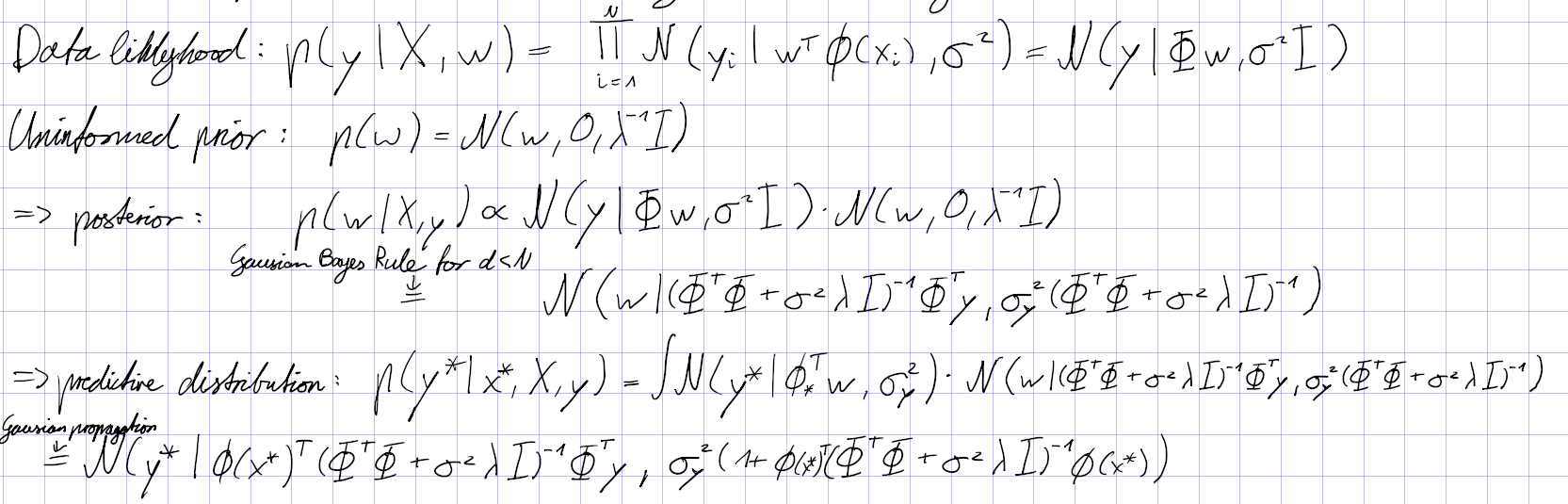
• What is the advantage of Bayesian Linear regression to Ridge regression? What is the conceptual difference?

  We not only obtain a point estimate, but a Gaussian distribution that quantifies the confidence we have at a prediction. It is computationally different, because for Bayesian Linear regression we are forced to invert matrices.

• What is the major advantage of GPs over Kernel Ridge Regression?

  We not only obtain a point estimate, but a Gaussian distribution that quantifies the confidence we have at a prediction.

• Why are GPs a Bayesian approach?

  Gaussian processes are just kernelized Bayesian Linear regression.

• What principle allowed deriving GPs from a Bayesian regression point of view?

  The kernel trick

Other questions

• What are possible interpretations of a maximum a-posteriori solution

  Interpolation between the MLE and a prior

  Bayesian learning, ignoring the uncertainty in the parameter vector

  Equivalent to ridge regression for Gaussian distributions with$\lambda_{ridge}=\lambda\sigma^2$

Lecture 8: Neural Networks

• How does logistic regression relate to neural networks?

  Neural networks are compositions of logistic regression functions (Perceptrons), sometimes swapping out the Sigmoid function for other activation functions

• What kind of functions can single layer neural networks learn?

  According to the representer theorem a NN with one hidden layer with infinite neurons is an arbitrary function approximator.

• Why do we need non-linear activation functions?

  Otherwise, we would have a composition of linear functions, which itself would be a linear function again.

• What activation functions can we use, and what are the advantages/disadvantages of those?

  • Sigmoid: Vanishing gradients, not zero centered, a bit expensive to compute, nice interpretation as probabilies

  • tanh: Vanishing gradients, zero centered, a bit expensive to compute

  • ReLU: No gradients for x < 0, efficient to compute, fast convergence in practice

  • Leaky ReLU/ PReLu: like ReLu, but meaningful gradients everywhere, fast convergence in practice

  • ELU: Vanishing gradients for x < 0, bit expensive to compute, fast convergence in practice

• What output layer and loss function to use given the task (regression, classification)?

  • Regression
    • Deterministic
      • Output Layer: Linear$W\boldsymbol{x} + \boldsymbol{b}$
      • Loss: Squared Error:$\frac{1}{2}(y_i-f(\boldsymbol{x}_i))^2$
    • Probabilistic
      • Output Layer: Linear Gaussian$\mathcal{N}(\boldsymbol{y}\mid W \boldsymbol{x} +\boldsymbol{b},\Sigma)$
      • Loss: Negative log likelihood$\mathcal{N}(y_i\mid \boldsymbol{\mu}(\boldsymbol{x}_i), \Sigma)$

  • Binary Classification
    • Deterministic
      • Output Layer: Linear$W\boldsymbol{x} + \boldsymbol{b}$
      • Loss: Hinge Loss$\max(0,1 - y_if(\boldsymbol{x}_i))$
    • Probabilistic
      • Output Layer: Sigmoid$\sigma(W\boldsymbol{x} + \boldsymbol{b} )$
      • Loss: Negative log-likelihood of Bernoulli$-c_i\log(f(\boldsymbol{x}_i)-(1-c_i)log(1-f(\boldsymbol{x}_i))$

  • Multi-class Classification
    • Deterministic
      • Output Layer: Linear$W\boldsymbol{x} + \boldsymbol{b}$
      • Loss:
    • Probabilistic
      • Output Layer: Softmax$\operatorname{softmax}(W\boldsymbol{x} + \boldsymbol{b} )$
      • Loss: Negative log-likelihood of multinomial:$-\sum_{k=1}^{K} \boldsymbol{h}_{c_{i}, k} \log y_{k}\left(\mathbf{x}_{i}\right)$

• Why not use a sigmoid activation function?

  Sigmoid has vanishing gradients and is therefore not suited for deeper neural networks where it is composed many times.

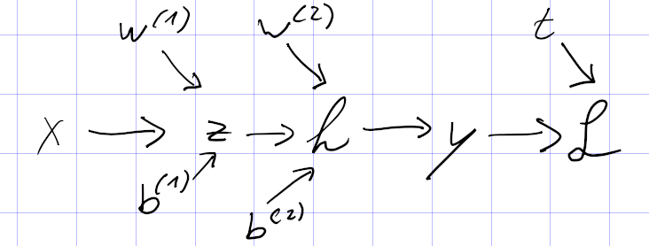
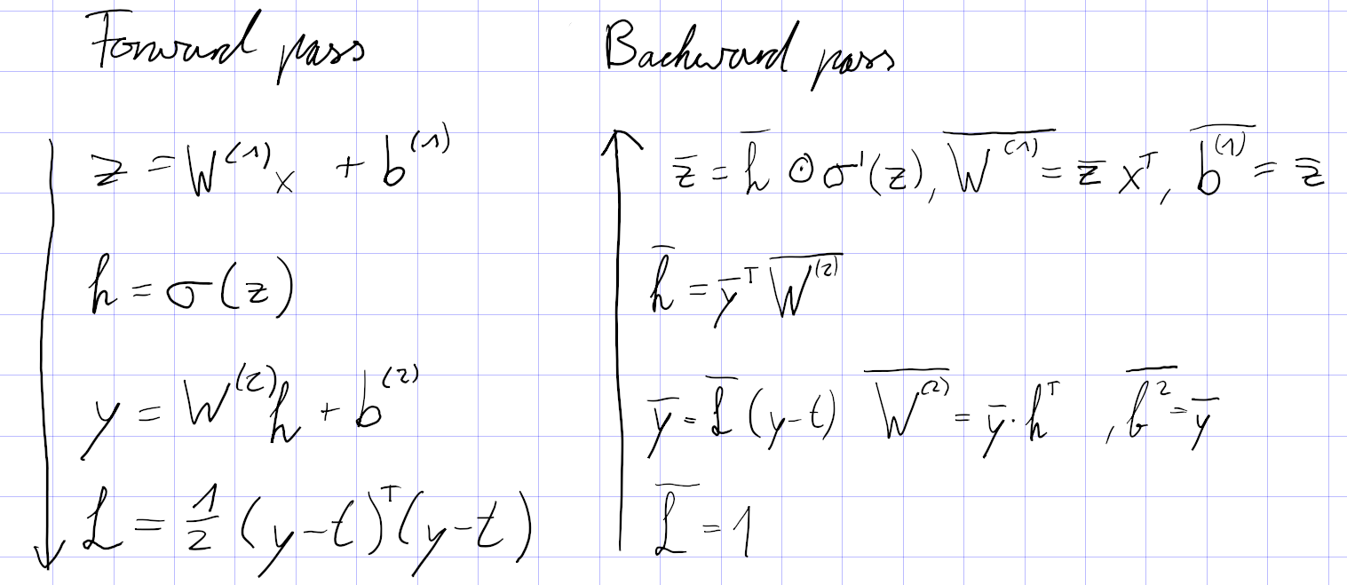
• Derive the equations for forward and backpropagation for a simple network

  For the multi layer perceptron from the slides:

  

  

• What is mini-batch gradient descent? Why use it instead of SGD or full gradient descent?

  Full gradient decent computes the gradients to updates weights and biases on the full training set, this is computationally expensive as it need to deal with huge matrices. SGD does single gradient steps for each sample, this is computationally less expensive, but introduces jitter in the descent, because one point is not a good representation of the whole dataset. Mini-batches is a tradeoff between both. The training set is partitioned into mini-batches (e.g., 32, 64 or 128 samples) in order to reduce jitter, but still be computationally tractable, especially with the parallelism of GPUs.

• Why neural networks can overfit, and what are the options to prevent it?

  Training a NN for to long reduces the training loss to a point where it does not reduce validation loss anymore. Especially NNs with many parameters have the capacity to store effectively training data. To prevent overfitting we can use classical approaches such as early stopping, weight regularization, ensembles or data augmentation, but also NN specific methods such as dropout and drop connect

• Why is the initialization of the network important?

  Different initializations tend to work better for activation functions. Due to vanishing gradients and different centers on the y-axis, the activations may vanish (only be meaningful for a narrow interval of inputs) the more layers we have.

• What can you read from the loss-curves during training (validation and training loss)?

  We can find see the areas at which the NN under fits (validation loss decreases) and overfits (validation loss increases) and the optimal point for stopping (local minimum of the validation loss). The training loss should always approach zero. If the training loss has too much jitter, we should decrease the learning rate. If it decreases too slowly, we should increase the learning rate. The training loss curve also gives us feedback for the effectiveness of a learning rate schedule.

• How can we accelerate gradient descent? How does Adam work?

  We can use second order methods. The most straight forward ones would be momentum or gradient normalization (RMSProp). Adam combines momentum and gradient normalization.

  $\begin{aligned} \boldsymbol{g}_{k} &=\nabla_{\boldsymbol{\theta}} \mathcal{L}\left(\boldsymbol{\theta}_{k}\right) \\ \boldsymbol{v}_{k+1, i} &=\gamma_{1} \boldsymbol{v}_{k, i}+\left(1-\gamma_{1}\right) \boldsymbol{g}_{k, i}^{2} \quad \ldots \text { gradient norm } \\ \boldsymbol{m}_{k+1} &=\gamma_{2} \boldsymbol{m}_{k}+\left(1-\gamma_{2}\right) \boldsymbol{g}_{k} \quad \ldots \text { momentum } \\ \boldsymbol{\theta}_{k+1, i} &=\boldsymbol{\theta}_{k, i}-\underbrace{\frac{\eta c_{2}(k)}{\sqrt{c_{1}(k) \boldsymbol{v}_{k+1, i}+\epsilon}}}_{\text {norm-based scaling }} \boldsymbol{m}_{k+1, i} \end{aligned}$

  We can also use learning rate decay, to make big steps at the beginning and then slow down.

Lecture 9: Convolutional Neural Networks and Recurrent Neural Networks

• Why are fully connected networks for images a bad idea, and why do we need images?

  Using fully connected networks would require us to have (width * height * channels) weights in the input layer. Also, by inputting the pixels as an array of numbers we throw away the spacial information in the image, because of the commutativity of the summation. The NN has to relearn the lost information.

  If the questions really intends to ask why we need images, the answer is obvious. Maybe it should read convolutions for images instead. In this case:

  We represent images as tensors [width, height, channels], and apply convolutions and pooling layers to reduce the number of input dimensions (= weights to train), while minimizing the (spacial) information we lose. Convolutions capture spacial information of neighboring pixels and the color channels of an image, by forming super-positions of pixels. Thinking of NNs as feature extractors, they help detect things like edges and shapes.

• What are the key components of a CNN?

  Convolutional layers, intermixed or just before, pooling layers, followed by fully connected layers. After convolutional layers and fully connected layers, activation functions are applied.

• What hyper-parameters can we set for a convolutional layer, and what is their meaning?

  Convolution window size F: How many pixels should we consider in the sliding window. Influencing what is considered local. Assumed to be quadratic.

  Number of filters K: How many convolution to apply. Can be interpreted as how many higher level feature types do we want to extract

  Stride S: Step size of the window, can be used to downscale output volume

  Padding: Size P (per side) and value of padding, commonly size is determined by filter size and stride and the value is zero.

• What hyper-parameters can we set for a pooling layer, and what is their meaning?

  Stride S: Step size of the window, can be used to downscale output volume. S ≠ 1 is much more common for pooling layers than for convolutional layers

  Window size F: How many pixels should we consider in the sliding window. Influencing what is considered local. Assumed to be quadratic.

• How can we compute the dimensionality of the output of a convolutional layer

  Input:$W_1\times H_1 \times D_1$

  Output:$W_2\times H_2 \times D_2;\;W_2=\frac{W_1 - F+2P}S+1;\;H_2=\frac{H_1-F+2P}S+1;\;D_2=K$

• Describe basic properties of AlexNet and VCG

  Using small but many convolutional layers and intermixing them with max-pooling and normalization. Followed by three densely connected layers.

• What is the main idea of ResNet to make it very deep?

  Introducing residual connection, that skip convolutions and just apply the identity functions. The result of the convolution is then combined with the identity. This can be interpreted as giving the layers not only one level of hierarchical feature extraction, but also access to lower level features. Also, the addition of input and output helps against vanishing gradients.

• How can we use CNNs with a “reasonable” amount of training data?

  With transfer learning we can use weights from a similar task and fine tune only the last few layers with a lower training rate.

• What are recurrent neural networks (RNNs) and why do we need them?

  Recurrent neural networks allow to handle sequential data (e.g., time series data) both as input and output. This is acheived by providing the network not only with a single data point (one time step) but also a state representing previous time steps.

• How do train a vanilla RNN?

  A vanilla RNN unit

  $\begin{aligned} \boldsymbol{h}_{t} &=\tanh \left(\boldsymbol{W}_{h h} \boldsymbol{h}_{t-1}+\boldsymbol{W}_{x h} \boldsymbol{x}_{t}\right) \\ &=\tanh \left(\boldsymbol{W}\left[\begin{array}{c} \boldsymbol{h}_{t-1} \\ \boldsymbol{x}_{t} \end{array}\right]\right) \end{aligned}$

  is trained with normal backpropagation

  $\frac{\partial \boldsymbol{h}_{t}}{\partial \boldsymbol{h}_{t-1}}=\operatorname{diag}\left(\tanh ^{\prime}\left(\boldsymbol{W}\left[\begin{array}{c} \boldsymbol{h}_{t-1} \\ \boldsymbol{x}_{t} \end{array}\right]\right)\right) \boldsymbol{W}_{h h}^{T}$

Lecture 10: Dimensionality Reduction and Clustering

• What does dimensionality reduction mean?

  Projecting data into a lower dimensional space, while minimizing the lost information.

• How does linear dimensionality reduction work?

  Let$D > M$. Given a data point$\boldsymbol{x}\in \mathbb{R}^D$ project it, using matrix$W\in \mathbb{R}^{M\times D}$, into a lower dimensional space$\boldsymbol{z}=W\boldsymbol{x}\in\mathbb{R}^M$. While maximizing the variance of thte projection

• What is PCA? What are the three things that it does?

  PCA stands for principal component analysis. It is a closed form method for linear dimensionality reduction. It allows us to control the lost variance in the data. Steps:

  Normalize the data (subtract the mean, usually also divide by the standard deviation)

  Do an eigendecomposition of the covariance matrix.

  Keep the basis eigenvectors corresponding to the largest eigenvalues.

  It guarantees:

  PCA maximizes variance of the projection

  PCA minimizes the error of the reconstruction

  PCA projects the data into a linear subspace

• What are the roles of the Eigenvectors and Eigenvalues in PCA?

  The eigenvalue$\lambda_i$ (of the centered covariance matrix) describes the marginal variance captured by the eigenvector$\boldsymbol{u}_i$.

• Can you describe applications of PCA?

  Image morphing, reducing input dimensionality for a machine learning algorithm (fewer weights to train for parametric algorithms, reduced curse of dimensionality effect for instance based algorithms that are using distances), image compression for certain types of images

• How is the clustering problem defined? Why is it called “unsupervised”?

  We are in the unsupervised setting, i.e. without having ground truth labels and want to group data points into distinct clusters. Clusters should be similar inside and dissimilar to other clusters.

• How do hierarchical clustering methods work? What is the rule of the cluster-2-cluster distance, and which distances can we use?

  Either bottom-up merging similar clusters together one level above, or top down by splitting clusters one level bellow. Algorithms for doing this or the cluster-2-cluster distance are not covered, but we whould use SLINK/CLINK/UPGMA for bottom up, measuring the cluster-2-cluster distance by:

  $\operatorname{dist}_{s l}(X, Y)=\min _{x \in X, y \in Y} \operatorname{dist}(x, y)$

  $\operatorname{dist}_{c l}(X, Y)=\max _{x \in X, y \in Y} \operatorname{dist}(x, y)$

  $\operatorname{dist}_{a l}(X, Y)=\frac{1}{|X| \cdot|Y|} \sum_{x \in X, y \in Y} \operatorname{dist}(x, y)$

  and DIANA for top down clustering

• How does the k-mean algorithm work? What are the 2 main steps?

  1. Place k center points randomly (on datapoints)

  2. Calculate the clostest center for each data point to get clusters

  3. Calculate the mean of each cluster, use the closest datapoint as center and go back to step 2.

• Why does the algorithm converge? What is it minimizing?

  K-means converges locally. Because in each iteration SDD is reduced and there is only a finite number of possible centers.

• Does k-means finds the global minimum of the objective?

  No. Minimizing$\sum_{i=1}^{n} \sum_{k} \mathbb{I}\left(z_{i}=k\right)d\left(\boldsymbol{x}_{i}, \boldsymbol{c}_{k}\right)^{2}$ is a NP-hard problem.

Lecture 11: Expectation Maximization

• What are mixture models?

  Linear combinations of distributions

  $p(\boldsymbol{x}) = \sum_{k=1}^{K}\pi_kp(\boldsymbol{x}\mid k)$

• Should gradient methods be used for training mixture models?

  No, because of the log of a sum for the negative loglikelihood, gradient decent is very slow.

• How does the EM algorithm work?

  Do some reasonable initialization of distribution parameters, e.g., with k-means

  Expectation: Compute cluster probabilities aka responsibilities for each sample (Bayes rule)$q_{i k}=p\left(k_{i}=k \mid \boldsymbol{x}_{i}\right)=\frac{p\left(\boldsymbol{x}_{i} \mid k\right) p(k)}{\sum_{j} p\left(\boldsymbol{x}_{i} \mid j\right) p(j)}=\frac{\pi_{k} \mathcal{N}\left(\boldsymbol{x}_{i} \mid \boldsymbol{\mu}_{k}, \boldsymbol{\Sigma}_{k}\right)}{\sum_{j=1}^{K} \pi_{j} \mathcal{N}\left(\boldsymbol{x}_{i} \mid \boldsymbol{\mu}_{j}, \boldsymbol{\Sigma}_{j}\right)}$

  Maximization: Compute (weighted) maximum likelihood estimate$\pi_{k}=\frac{\sum_{i} q_{i k}}{N} \quad \boldsymbol{\mu}_{k}=\frac{\sum_{i} q_{i k} \boldsymbol{x}_{i}}{\sum_{i} q_{i k}} \quad{\Sigma}_{k}=\frac{\sum_{i} q_{i k}\left(\boldsymbol{x}_{i}-\boldsymbol{\mu}_{k}\right)\left(\boldsymbol{x}_{i}-\boldsymbol{\mu}_{k}\right)^{T}}{\sum_{i} q_{i k}}$

• What is the biggest problem of mixture models?

  We are left with the model selection problem of choosing the number and kind of distributions to mix.

• How does EM decomposes the marginal likelihood?

  $\log p(\boldsymbol{x} \mid \boldsymbol{\theta})=\mathcal{L}(q, \boldsymbol{\theta})+\mathrm{KL}(q(z) \| p(z \mid \boldsymbol{x}))$

• Why does EM always improve the lower bound?

  In the expectation step, we minimize the second term of the marginal log likelihood$\log p(\boldsymbol{x} \mid \boldsymbol{\theta})=\mathcal{L}(q, \boldsymbol{\theta})+\mathrm{KL}(q(z) \| p(z \mid \boldsymbol{x}))$ without changing the marginal, as it does not depend on$q$. Therefore, the lower bound increases. The maximization step explicitly maximizes the lower bound directly.

• Why does EM always improve the marginal likelihood?

  In the previous answer, we argued, that the expectation step does not change the marginal likelihood. In the maximization step, z we increase the lower bound and the KL, as the KL can’t get smaller than zero.

• Why can we optimize each mixture component independently with EM

  We have independent loss functions for every component k, because the M-step gives us just the sum of the components.

  $\boldsymbol{\theta}=\underset{\boldsymbol{\theta}}{\arg \max } \sum_{i} \sum_{k} q_{i k} \log p(k) p\left(\boldsymbol{x}_{i} \mid k\right)$

• Why do we need sampling for continuous latent variables?

  Because there is usually no analytical solution for the lower bound integral

  $\sum_{i}\left(\int_{z} q_{i}(z) \log p\left(\boldsymbol{x}_{i}, z \mid \boldsymbol{\theta}\right) d z-\int_{z} q_{i}(z) \log q_{i}(z) d z\right)$, we do a monte carlo estimation of it.